verhelv

@bucky, Sorry dat ik het zo snel had afgesloten. Ik wist sowieso niet van een dubbel topic.. Ik ben niet echt gewend om op forums te werken. Alleszins dank voor iedere input die me wijzer maakt

hallo, op aanvraag van Alpha hierbij mijn oplossing. Die komt ongeveer overeen met jou oplossing. ipv het in één formule te willen proppen heb ik gefaseerd gewerkt. op basis van de lijst productoverview heb ik de verkochte productcodes gekopieerd. Eerst per reeks kolommen in bereik product_info met sommen.als (voorwaarde gelijk aan "eu"/"world"; voorwaarde gelijk aan "productcode" de aantallen verkochte codes opgezocht. Als je een beetje met excel kan werken zet je er 1x de formules "eu"/"world" in en kan je dan eerst per rij kopiëren. Daarna versleuteling aanpassen en dan naar beneden kopiëren. Dan per aanwezige productcode voor de bekomen rijen de totaalsom "eu" en als "world" in formule gegoten. som(van de kolommen eu/world) per productcode. De verkregen info per werkmap (datumsheets)heb ik dan gekoppeld in een andere werkmap waarop ik opnieuw met som.als(voorwaarde gelijk aan "productcode") een volledig totaalsom kon bekomen per productcode verkocht in de maand februari.+ de totaalwaarden "eu" en "world" kan berekenen. Alleen goed opletten dat mijn formules overal juist staan en de juiste return geven. En genoeg beveiligen Ik zou wel met VBA willen werken maar dan moet ik eerst op cursus vrees ik.

bedankt voor de hulp maar ik ben eruit.. beetje faseren en dan kom ik er. Teveel in 1 formule willen stoppen is niet altijd the easy way! Veerle

Txs bucky. ik heb de punten vervangen door "," Echter maak jij de som van total items waar ik een som nodig heb van Product_items in bereik "Product_info" als een bvb. productcode 28072 voorkomt. dus als in Product_info productcode 28072 voorkomt wil ik dat hij het getal in de 2de kolom erop volgend optelt. Daarna kan ik de splitsing eu/world maken. Veerle

Hallo, ik zou een overzicht moeten verkrijgen van de aantallen verkochte productitems per productcodes uit sheet "ordertemplate" en dit verdeeld over "region" EU/World. De moeilijkheid zit hem erin dat de productcode zich op verschillende cellen binnen het bereik met voorgedefineerde naam "Product_info" kunnen bevinden en ik steeds de cel in de 2de kolom na de cel met die productcode moet optellen. DUS: als region = EU dan aantal product_items per productcode (zelfde voor region world) Een 2de moeilijkheid is dat ik tot de totaalsom moet komen van alle werkmappen aangemaakt voor de maand. Als ik dit met formules moet doen zijn deze ellenlang en met VBA werk ik niet. Heb al even acces bekeken maar ik geraak er niet. vb excel template in bijlage zoals deze binnenkomen. na mij drie dagen suf peinzen toch op zoek naar hulp :-( 20160201 ORDERS adapted docs.xlsx

Hallo, ik zou een overzicht moeten verkrijgen van de aantallen verkochte productitems per productcodes uit sheet "ordertemplate" en dit verdeeld over "region" EU/World. De moeilijkheid zit hem erin dat de productcode zich op verschillende cellen binnen het bereik met voorgedefineerde naam "Product_info" kunnen bevinden en ik steeds de cel in de 2de kolom na de cel met die productcode moet optellen. DUS: als region = EU dan aantal product_items per productcode (zelfde voor region world) Een 2de moeilijkheid is dat ik tot de totaalsom moet komen van alle werkmappen aangemaakt voor de maand. Als ik dit met formules moet doen zijn deze ellenlang en met VBA werk ik niet. Heb al even acces bekeken maar ik geraak er niet. vb excel template in bijlage zoals deze binnenkomen. na mij drie dagen suf peinzen toch op zoek naar hulp :-(

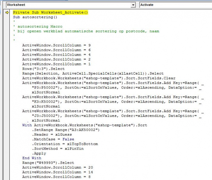
txs, but.. neen zo voorkom ik het probleem niet van de autonummering bij sortering. ik heb de opmaak van autonummering aangepast zodat bij sortering de nummer behouden blijft. Tenzij men de kolom selecteert natuurlijk. Met die reden wou ik die autsortering zodat het steeds juist verloopt en de lijst na aanvulling altijd gesorteerd blijft. Hierbij de excel template met VBA ingevoegd: vb excelforum.xlsm

ik probeer mijn aanpak aan te passen en uit utopia te geraken. mijn volgend plan: de autonummering zal niet op rijnummer worden gecreëerd maar op ingevuld cijfer. (manueel dus) om het foutief sorteren tegen te gaan wil ik dan wel een autosorting inzetten met VBA bij het openen van het werkblad. Wat doe ik fout? v. Excel een uitdaging om niet uit de weg te gaan - - - Updated - - - zij is een zij die een hij heeft laten staan (profiel).

idd. zij wil dat het nummer gecreëerd in kolom B eigen blijft aan de gegevens nu verder ingevuld op dezelfde rij. Maar ik vrees dat ik in utopie leef of anders te werk zal moeten gaan. V. - - - Updated - - - plx, dit is de opbouw van een database register (kopie). de velden vanaf kolom D zijn invulvelden. Die kringverwijzingen zijn er omdat het een kopie is. Het resultaat heb ik nl. de autonummering in kolom B Maar deze moet genesteld zijn aan de gegevens ingevuld kolom I tot .. zodat bij sortering het nummer genesteld zit aan de gegevens in kolom I tot.. snap je me? sorry, mijn computertaal kan er soms al eens naast zitten V.

ja dat ken ik maar dan heb ik weer een probleem. Het zou echt vanaf invullen geblokkeerd moeten staan. toch bedankt voor de reactie V.

hallo, ik wil in excel een autonummering (Kolom opmaken. Dat is gelukt aan de hand van de een optelnummering (Kolom A). Doch wil ik dat de autonummering gekoppeld blijft aan de gegevens in deze rij. ik kan blad beveiligen tegen verwijderen rij maar wat als men zou Albabetisch sorteren of... vb bijlage : akkkk moet het nummer OFL 13-010003 behouden ook als men per ongeluk op kolomselectie zou selecteren. Dit nummer is een uniek gelinkte referentie. hopelijk ben ik duidelijk. Niet sorteren is geen optie want het is voor een brede Database. merciekes. V. opvolgnummers excel vastzetten.xlsx

Bucky, Bedankt om dit te willen bekijken. hierbij een voorbeeld: [TABLE=width: 1013] [TR] [TD=class: xl63, width: 64, bgcolor: transparent][/TD] [TD=class: xl63, width: 65, bgcolor: transparent][/TD] [TD=class: xl63, width: 64, bgcolor: transparent][/TD] [TD=class: xl70, width: 87, bgcolor: transparent]Bestellingnr. [/TD] [TD=class: xl63, width: 79, bgcolor: transparent]klantnr. [/TD] [TD=class: xl63, width: 64, bgcolor: transparent]Klant [/TD] [TD=class: xl63, width: 87, bgcolor: transparent]Aangemaakt [/TD] [TD=class: xl63, width: 59, bgcolor: transparent]Aangemaakt door [/TD] [TD=class: xl63, width: 62, bgcolor: transparent]Aangemaakt Gebruiker [/TD] [TD=class: xl63, width: 75, bgcolor: transparent]Einddatum [/TD] [TD=width: 65, bgcolor: transparent][/TD] [TD=width: 65, bgcolor: transparent][/TD] [TD=width: 65, bgcolor: transparent][/TD] [TD=width: 65, bgcolor: transparent][/TD] [TD=width: 64, bgcolor: transparent][/TD] [TD=width: 64, bgcolor: transparent][/TD] [TD=width: 64, bgcolor: transparent][/TD] [TD=width: 64, bgcolor: transparent][/TD] [TD=width: 64, bgcolor: transparent][/TD] [TD=width: 64, bgcolor: transparent][/TD] [/TR] [TR] [TD=class: xl66, bgcolor: #99ff33][/TD] [TD=class: xl66, bgcolor: #99ff33][/TD] [TD=class: xl66, bgcolor: #99ff33][/TD] [TD=class: xl75, bgcolor: #99ff33]1000 [/TD] [TD=class: xl66, bgcolor: #99ff33, align: right]105 [/TD] [TD=class: xl66, bgcolor: #99ff33]peeters [/TD] [TD=class: xl68, bgcolor: #99ff33, align: right]26-04-2012 [/TD] [TD=class: xl74, bgcolor: #99ff33]xxxxxxx [/TD] [TD=class: xl74, bgcolor: #99ff33]xxxxxxx [/TD] [TD=class: xl68, bgcolor: #99ff33, align: right]26-04-2012 [/TD] [TD=class: xl66, bgcolor: #99ff33, align: right]1 [/TD] [TD=class: xl77, bgcolor: transparent, align: right]2 [/TD] [TD=class: xl77, bgcolor: transparent, colspan: 8]formule CT niet correct want geeft resultaat op alle lijnen ook dubbel D -gegevens [/TD] [/TR] [TR] [TD=class: xl66, bgcolor: #99ff33][/TD] [TD=class: xl66, bgcolor: #99ff33][/TD] [TD=class: xl66, bgcolor: #99ff33][/TD] [TD=class: xl72, bgcolor: #99ff33]1001 [/TD] [TD=class: xl66, bgcolor: #99ff33, align: right]106 [/TD] [TD=class: xl74, bgcolor: #99ff33]wauters [/TD] [TD=class: xl68, bgcolor: #99ff33, align: right]26-04-2012 [/TD] [TD=class: xl74, bgcolor: #99ff33]xxxxxxx [/TD] [TD=class: xl74, bgcolor: #99ff33]xxxxxxx [/TD] [TD=class: xl68, bgcolor: #99ff33, align: right]26-04-2012 [/TD] [TD=class: xl66, bgcolor: #99ff33, align: right]1 [/TD] [TD=class: xl77, bgcolor: transparent, align: right]1 [/TD] [TD=bgcolor: transparent][/TD] [TD=bgcolor: transparent][/TD] [TD=bgcolor: transparent][/TD] [TD=bgcolor: transparent][/TD] [TD=bgcolor: transparent][/TD] [TD=bgcolor: transparent][/TD] [TD=bgcolor: transparent][/TD] [TD=bgcolor: transparent][/TD] [/TR] [TR] [TD=class: xl66, bgcolor: #99ff33][/TD] [TD=class: xl66, bgcolor: #99ff33][/TD] [TD=class: xl66, bgcolor: #99ff33][/TD] [TD=class: xl76, bgcolor: #99ff33]1000 [/TD] [TD=class: xl66, bgcolor: #99ff33, align: right]107 [/TD] [TD=class: xl74, bgcolor: #99ff33]wouters [/TD] [TD=class: xl68, bgcolor: #99ff33, align: right]26-04-2012 [/TD] [TD=class: xl74, bgcolor: #99ff33]xxxxxxx [/TD] [TD=class: xl74, bgcolor: #99ff33]xxxxxxx [/TD] [TD=class: xl68, bgcolor: #99ff33, align: right]26-04-2012 [/TD] [TD=class: xl66, bgcolor: #99ff33, align: right]1 [/TD] [TD=class: xl77, bgcolor: transparent, align: right]2 [/TD] [TD=bgcolor: transparent][/TD] [TD=bgcolor: transparent][/TD] [TD=bgcolor: transparent][/TD] [TD=bgcolor: transparent][/TD] [TD=bgcolor: transparent][/TD] [TD=bgcolor: transparent][/TD] [TD=bgcolor: transparent][/TD] [TD=bgcolor: transparent][/TD] [/TR] [TR] [TD=class: xl66, bgcolor: #99ff33][/TD] [TD=class: xl66, bgcolor: #99ff33][/TD] [TD=class: xl66, bgcolor: #99ff33][/TD] [TD=class: xl73, bgcolor: #99ff33][/TD] [TD=class: xl66, bgcolor: #99ff33, align: right]105 [/TD] [TD=class: xl74, bgcolor: #99ff33]willems [/TD] [TD=class: xl68, bgcolor: #99ff33, align: right]26-04-2012 [/TD] [TD=class: xl74, bgcolor: #99ff33]xxxxxxx [/TD] [TD=class: xl74, bgcolor: #99ff33]xxxxxxx [/TD] [TD=class: xl68, bgcolor: #99ff33, align: right]26-04-2012 [/TD] [TD=class: xl66, bgcolor: #99ff33, align: right]1 [/TD] [TD=class: xl77, bgcolor: transparent, align: right]0 [/TD] [TD=bgcolor: transparent][/TD] [TD=bgcolor: transparent][/TD] [TD=bgcolor: transparent][/TD] [TD=bgcolor: transparent][/TD] [TD=bgcolor: transparent][/TD] [TD=bgcolor: transparent][/TD] [TD=bgcolor: transparent][/TD] [TD=bgcolor: transparent][/TD] [/TR] [TR] [TD=class: xl66, bgcolor: #99ff33][/TD] [TD=class: xl66, bgcolor: #99ff33][/TD] [TD=class: xl66, bgcolor: #99ff33][/TD] [TD=class: xl73, bgcolor: #99ff33][/TD] [TD=class: xl66, bgcolor: #99ff33, align: right]106 [/TD] [TD=class: xl74, bgcolor: #99ff33]willems [/TD] [TD=class: xl68, bgcolor: #99ff33, align: right]27-04-2012 [/TD] [TD=class: xl74, bgcolor: #99ff33]xxxxxxx [/TD] [TD=class: xl74, bgcolor: #99ff33]xxxxxxx [/TD] [TD=class: xl68, bgcolor: #99ff33, align: right]27-04-2012 [/TD] [TD=class: xl66, bgcolor: #99ff33, align: right]1 [/TD] [TD=class: xl77, bgcolor: transparent, align: right]0 [/TD] [TD=bgcolor: transparent][/TD] [TD=bgcolor: transparent][/TD] [TD=bgcolor: transparent][/TD] [TD=bgcolor: transparent][/TD] [TD=bgcolor: transparent][/TD] [TD=bgcolor: transparent][/TD] [TD=bgcolor: transparent][/TD] [TD=bgcolor: transparent][/TD] [/TR] [TR] [TD=bgcolor: transparent][/TD] [TD=bgcolor: transparent][/TD] [TD=bgcolor: transparent][/TD] [TD=bgcolor: transparent][/TD] [TD=bgcolor: transparent][/TD] [TD=bgcolor: transparent][/TD] [TD=bgcolor: transparent][/TD] [TD=bgcolor: transparent][/TD] [TD=bgcolor: transparent][/TD] [TD=bgcolor: transparent][/TD] [TD=bgcolor: transparent][/TD] [TD=bgcolor: transparent][/TD] [TD=bgcolor: transparent][/TD] [TD=bgcolor: transparent][/TD] [TD=bgcolor: transparent][/TD] [TD=bgcolor: transparent][/TD] [TD=bgcolor: transparent][/TD] [TD=bgcolor: transparent][/TD] [TD=bgcolor: transparent][/TD] [TD=bgcolor: transparent][/TD] [/TR] [TR] [TD=bgcolor: transparent][/TD] [TD=class: xl69, bgcolor: transparent, colspan: 96]ik wil dat hij doorlooptijd van bestelling D2 geeft echter is zelfde bestelling behandeld door andere dienst zie D4. [/TD] [TD=bgcolor: transparent][/TD] [TD=bgcolor: transparent][/TD] [TD=bgcolor: transparent][/TD] [TD=bgcolor: transparent][/TD] [TD=bgcolor: transparent][/TD] [TD=bgcolor: transparent][/TD] [TD=bgcolor: transparent][/TD] [TD=bgcolor: transparent][/TD] [TD=bgcolor: transparent][/TD] [/TR] [TR] [TD=bgcolor: transparent][/TD] [TD=class: xl69, bgcolor: transparent, colspan: 5]hij moet dus CS2+CS4 doen maar enkel vermelden op lijn 2 [/TD] [TD=bgcolor: transparent][/TD] [TD=bgcolor: transparent][/TD] [TD=bgcolor: transparent][/TD] [TD=bgcolor: transparent][/TD] [TD=bgcolor: transparent][/TD] [TD=bgcolor: transparent][/TD] [TD=bgcolor: transparent][/TD] [TD=bgcolor: transparent][/TD] [TD=bgcolor: transparent][/TD] [TD=bgcolor: transparent][/TD] [TD=bgcolor: transparent][/TD] [TD=bgcolor: transparent][/TD] [TD=bgcolor: transparent][/TD] [TD=bgcolor: transparent][/TD] [/TR] [TR] [TD=bgcolor: transparent][/TD] [TD=bgcolor: transparent][/TD] [TD=bgcolor: transparent][/TD] [TD=bgcolor: transparent][/TD] [TD=bgcolor: transparent][/TD] [TD=bgcolor: transparent][/TD] [TD=bgcolor: transparent][/TD] [TD=bgcolor: transparent][/TD] [TD=bgcolor: transparent][/TD] [TD=bgcolor: transparent][/TD] [TD=bgcolor: transparent][/TD] [TD=bgcolor: transparent][/TD] [TD=bgcolor: transparent][/TD] [TD=bgcolor: transparent][/TD] [TD=bgcolor: transparent][/TD] [TD=bgcolor: transparent][/TD] [TD=bgcolor: transparent][/TD] [TD=bgcolor: transparent][/TD] [TD=bgcolor: transparent][/TD] [TD=bgcolor: transparent][/TD] [/TR] [TR] [TD=bgcolor: transparent][/TD] [TD=class: xl69, bgcolor: transparent, colspan: 14]om correct te werken mag hij in die berekening cel D5 niet meenemen want anders [/TD] [TD=bgcolor: transparent][/TD] [TD=bgcolor: transparent][/TD] [TD=bgcolor: transparent][/TD] [TD=bgcolor: transparent][/TD] [TD=bgcolor: transparent][/TD] [TD=bgcolor: transparent][/TD] [TD=bgcolor: transparent][/TD] [TD=bgcolor: transparent][/TD] [TD=bgcolor: transparent][/TD] [TD=bgcolor: transparent][/TD] [TD=bgcolor: transparent][/TD] [TD=bgcolor: transparent][/TD] [/TR] [TR] [TD=bgcolor: transparent][/TD] [TD=bgcolor: transparent][/TD] [TD=bgcolor: transparent][/TD] [TD=bgcolor: transparent][/TD] [TD=bgcolor: transparent][/TD] [TD=bgcolor: transparent][/TD] [TD=bgcolor: transparent][/TD] [TD=bgcolor: transparent][/TD] [TD=bgcolor: transparent][/TD] [TD=bgcolor: transparent][/TD] [TD=bgcolor: transparent][/TD] [TD=bgcolor: transparent][/TD] [TD=bgcolor: transparent][/TD] [TD=bgcolor: transparent][/TD] [TD=bgcolor: transparent][/TD] [TD=bgcolor: transparent][/TD] [TD=bgcolor: transparent][/TD] [TD=bgcolor: transparent][/TD] [TD=bgcolor: transparent][/TD] [TD=bgcolor: transparent][/TD] [/TR] [TR] [TD=bgcolor: transparent][/TD] [TD=class: xl69, bgcolor: transparent, colspan: 5]in mijn ander rapport doet hij dit voor de lege velden: [/TD] [TD=class: xl69, bgcolor: transparent, colspan: 4]in CT resultaat 85 = som van alle lege cellen [/TD] [TD=bgcolor: transparent][/TD] [TD=bgcolor: transparent][/TD] [TD=bgcolor: transparent][/TD] [TD=bgcolor: transparent][/TD] [TD=bgcolor: transparent][/TD] [TD=bgcolor: transparent][/TD] [TD=bgcolor: transparent][/TD] [TD=bgcolor: transparent][/TD] [TD=bgcolor: transparent][/TD] [TD=bgcolor: transparent][/TD] [/TR] [TR] [TD=bgcolor: transparent][/TD] [TD=bgcolor: transparent][/TD] [TD=bgcolor: transparent][/TD] [TD=bgcolor: transparent][/TD] [TD=class: xl71, bgcolor: transparent][/TD] [TD=bgcolor: transparent][/TD] [TD=bgcolor: transparent][/TD] [TD=class: xl64, bgcolor: transparent][/TD] [TD=bgcolor: transparent][/TD] [TD=bgcolor: transparent][/TD] [TD=class: xl65, bgcolor: transparent][/TD] [TD=bgcolor: transparent][/TD] [TD=bgcolor: transparent][/TD] [TD=bgcolor: transparent][/TD] [TD=bgcolor: transparent][/TD] [TD=bgcolor: transparent][/TD] [TD=bgcolor: transparent][/TD] [TD=bgcolor: transparent][/TD] [TD=bgcolor: transparent][/TD] [TD=bgcolor: transparent][/TD] [/TR] [/TABLE]

hallo, ik heb even hulp nodig. Ik ben nog een nitwit in de wereld van formules en probeer het volgende te bekomen: als er zich dubbel waarden in kolom D bevinden moet ik de som krijgen van kolom CS maar maar 1 keer laten voorkomen. Hierbij moeten de lege velden in kolom D genegeerd worden. zover was ik gekomen: =SOM.ALS($D$2:$D2;D2;CS:CS) ik moet echter nog checken dat ik op het goede spoor zit. de lege velden worden niet genegeerd. Ik ben nu al de hele avond met ALS en EN functie aan het 'knoefelen' maar ik kom niet tot een goede formulexD is er iemand die mijn chinees begrijpt en mij verder wil helpen?? groetjes, Me ---------- Post toegevoegd om 21:17 ---------- Vorige post was om 21:07 ---------- =SOM.ALS($D$2:$D2;D2;CS:CS) deze formule klopt ook niet..